ModelOrderReduction.jl

ModelOrderReduction.jl is a package for automatically reducing the computational complexity of mathematical models, while keeping expected fidelity within a controlled error bound. These methods construct a submodel via a projection where solving the smaller model gives approximate information about the full model. MOR.jl uses ModelingToolkit.jl as a system description and automatically transforms equations to the subform, defining the observables to automatically lazily reconstruct the full model on-demand in a fast and stable form.

Tutorials and Documentation

For information on using the package, see the stable documentation. Use the in-development documentation for the version of the documentation, which contains the unreleased features.

Example

Proper Orthogonal Decomposition (POD) Galerkin on an array ODE

using ModelingToolkit, OrdinaryDiffEq, ModelOrderReduction
import SymbolicIndexingInterface as SII

@independent_variables t
@variables z(t)[1:32]
z_scalars = ModelingToolkit.Symbolics.value.(ModelingToolkit.Symbolics.scalarize(z))
D = Differential(t)
z0 = [sin(0.3 * i) for i in 1:32]
@named sys = System(
    [D(z) ~ -z - z .^ 3], t, z_scalars, [];
    initial_conditions = [z => z0, D(z) => -z0 - z0 .^ 3],
)
full_prob = DAEProblem(complete(sys), nothing, (0.0, 1.0); build_initializeprob = false)
sol = solve(full_prob)

# POD Galerkin: one array reduced equation, O(1) symbolic residual in the grid size
rom = pod(full_prob, sol, 4)
rom_prob = DAEProblem(rom, nothing; build_initializeprob = false)
rom_sol = solve(rom_prob)
z_approx = [SII.observed(rom, z)(u, rom_prob.p, tt) for (u, tt) in zip(rom_sol.u, rom_sol.t)]

For nonlinear systems where the online residual must also stay independent of the grid, use deim (POD with Discrete Empirical Interpolation).

Proper Orthogonal Decomposition and Discrete Empirical Interpolation Method (POD-DEIM) on the FitzHugh-Nagumo system

using ModelingToolkit, MethodOfLines, DifferentialEquations, ModelOrderReduction
using SciMLBase: discretize

# firstly construct a ModelingToolkit.PDESystem for the FitzHugh-Nagumo model
@independent_variables x t
@variables v(..) w(..)
Dx = Differential(x)
Dxx = Dx^2
Dt = Differential(t)
const L = 1.0
const ε = 0.015
const b = 0.5
const γ = 2.0
const c = 0.05
f(v) = v * (v - 0.1) * (1.0 - v)
i₀(t) = 50000.0t^3 * exp(-15.0t)
eqs = [ε * Dt(v(x, t)) ~ ε^2 * Dxx(v(x, t)) + f(v(x, t)) - w(x, t) + c,
    Dt(w(x, t)) ~ b * v(x, t) - γ * w(x, t) + c]
bcs = [v(x, 0.0) ~ 0.0, w(x, 0) ~ 0.0, Dx(v(0, t)) ~ -i₀(t), Dx(v(L, t)) ~ 0.0]
domains = [x ∈ (0.0, L), t ∈ (0.0, 14.0)]
ivs = [x, t]
dvs = [v(x, t), w(x, t)]
pde_sys = PDESystem(eqs, bcs, domains, ivs, dvs; name = Symbol("FitzHugh-Nagumo"))

# discretize to MethodOfLines v1's array-form DAEProblem
N = 15 # equidistant discretization intervals
dx = (L - 0.0) / N
dxs = [x => dx]
discretization = MOLFiniteDifference(dxs, t)
full_prob = discretize(pde_sys, discretization; fallback = false)

# solve the full-order model to get snapshots
sol = solve(full_prob)

# set POD and DEIM dimensions
# apply POD-DEIM to obtain the reduced-order model
pod_dim = deim_dim = 5
deim_sys = deim(full_prob, sol, pod_dim; deim_dim = deim_dim)
deim_prob = DAEProblem(deim_sys, nothing; build_initializeprob = false)
deim_sol = solve(deim_prob)

# retrieve the approximate solution of the original full-order model
sol_deim_x = deim_sol[x]
sol_deim_v = deim_sol[v(x, t)]
sol_deim_w = deim_sol[w(x, t)]

The following figure shows the comparison of the solutions of the 32-dimension full-order model and the POD5-DEIM5 reduced-order model.

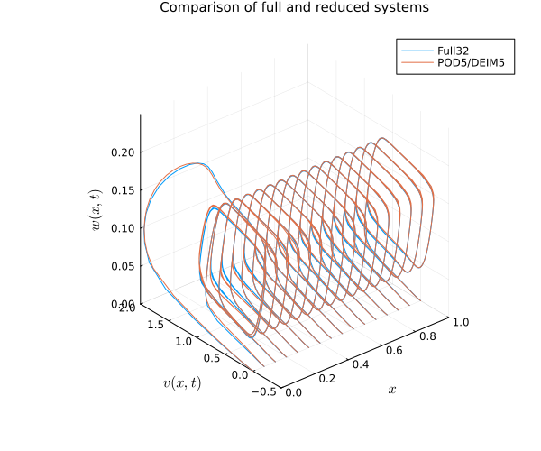
For fixed reduced dimensions, field and forcing structure, and local nonlinear stencils, the reduced dynamics and field reconstruction use a grid-independent symbolic array graph. Offline reduction and full-field reconstruction still scale with the grid. See the tutorial for the algebraic reconstruction approximation and supported DAE scope.